Model Representation
Recall that in regression problems, we are taking input variables and trying to map the output onto a continuous expected result function.
Linear regression with one variable is also known as "univariate linear regression."
Univariate linear regression is used when you want to predict a single output value from a single input value. We're doing supervised learning here, so that means we already have an idea what the input/output cause and effect should be.
The Hypothesis Function
Our hypothesis function has the general form:
\(h_θ(x)=θ_0+θ_1x\)
We give to \(h_θ\) values for \(θ_0\) and \(θ_1\) to get our output '\(y\)'. In other words, we are trying to create a function called \(h_θ\) that is able to reliably map our input data (the x's) to our output data (the y's).
Example: | x (input) | y (output)| | :--- | :--- | | 0 | 4 | | 1 | 7 | | 2 | 7| | 3 | 8|
Now we can make a random guess about our \(h_θ\) function: \(θ_0=2\) and \(θ_1=2\). The hypothesis function becomes \(h_θ(x)=2+2x\).
So for input of 1 to our hypothesis, y will be 4. This is off by 3.
Cost Function
We can measure the accuracy of our hypothesis function by using a cost function. This takes an average (actually a fancier version of an average) of all the results of the hypothesis with inputs from x's compared to the actual output y's.
\(J(θ_0,θ_1)=\frac{1}{2m}∑_{i=1}^{m}(h_θ(x_i)−y_i)^2\)
To break it apart, it is \(\frac{1}{2}\overline{x}\) where \(\overline{x}\) is the mean of the squares of \(h_θ(x_i) - y_i\), or the difference between the predicted value and the actual value.
This function is otherwise called the "Squared error function", or Mean squared error(均方误差). The mean is halved \((\frac{1}{2m})\) as a convenience for the computation of the gradient descent(梯度下降), as the derivative(导数) term of the square function will cancel out the \(\frac{1}{2}\) term.
Now we are able to concretely measure the accuracy of our predictor function against the correct results we have so that we can predict new results we don't have.
Gradient Descent
So we have our hypothesis function and we have a way of measuring how accurate it is. Now what we need is a way to automatically improve our hypothesis function. That's where gradient descent comes in.
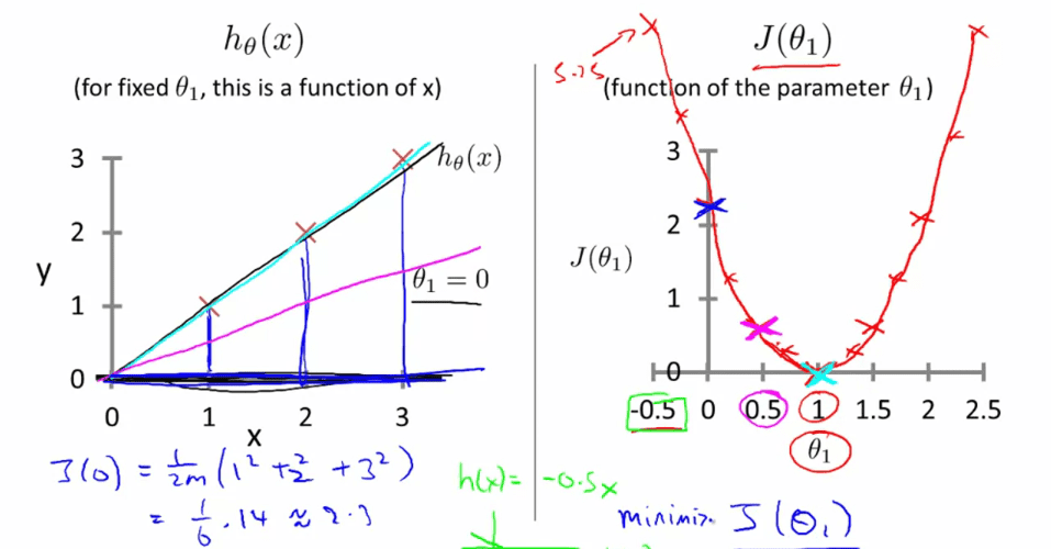
Imagine that we graph our hypothesis function based on its fields \(θ_0\) and \(θ_1\) (actually we are graphing the cost function for the combinations of parameters). This can be kind of confusing; we are moving up to a higher level of abstraction. We are not graphing x and y itself, but the guesses of our hypothesis function.
We put \(θ_0\) on the x axis and \(θ_1\) on the z axis, with the cost function on the vertical y axis. The points on our graph will be the result of the cost function using our hypothesis with those specific theta parameters.
We will know that we have succeeded when our cost function is at the very bottom of the pits in our graph, i.e. when its value is the minimum.
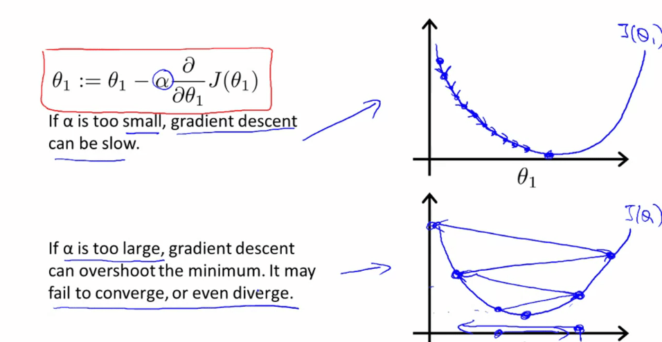
The way we do this is by taking the derivative (the line tangent to a function) of our cost function. The slope of the tangent is the derivative at that point and it will give us a direction to move towards. We make steps down that derivative by the parameter \(α\), called the learning rate.
The gradient descent equation is:
repeat until convergence(收敛):{ \(θ_j : = θ_j − α \frac{∂}{∂θ_j}J(θ_0,θ_1)\) for j=0 and j=1 }
Intuitively, this could be thought of as:
repeat until convergence:{ \(θ_j : = θ_j − α\)[Slope of tangent aka derivative] }
Simultaneous update
\(temp0 := \theta - \alpha\frac{\partial}{\partial\theta_0}J(\theta_0, \theta_1)\) \(temp1 := \theta - \alpha\frac{\partial}{\partial\theta_1}J(\theta_0, \theta_1)\) \(\theta_0 := temp0\) \(\theta_1 := temp1\)
Learning rate \(\alpha\)
Gradient Descent for Linear Regression
When specifically applied to the case of linear regression, a new form of the gradient descent equation can be derived. We can substitute our actual cost function and our actual hypothesis function and modify the equation to (the derivation of the formulas are out of the scope of this course, but a really great one can be found here:
repeat until convergence: { \(θ_0 : = θ_0 − α\frac{1}{m}∑_{i=1}^{m}(h_θ(x_i)−y_i)\) \(θ_1 : = θ_1 − α\frac{1}{m}∑_{i=1}^{m}(h_θ(x_i)−y_i)x_i\) }
where \(m\) is the size of the training set, \(θ_0\) a constant that will be changing simultaneously with \(θ_1\) and \(x_i,y_i\) are values of the given training set.
Note that we have separated out the two cases for \(θ_j\) and that for \(θ_1\) we are multiplying \(x_i\) at the end due to the derivative.
The point of all this is that if we start with a guess for our hypothesis and then repeatedly apply these gradient descent equations, our hypothesis will become more and more accurate.
Batch Gradient Descent
Batch : Each step of gradient descent uses all the training examples.
What's Next
Instead of using linear regression on just one input variable, we'll generalize and expand our concepts so that we can predict data with multiple input variables. Also, we'll solve for \(θ_0\) and \(θ_1\) exactly without needing an iterative function like gradient descent.